TRUNCATION ERRORS IN THE MODAL VIBRATION ANALYSIS OF THE ROTOR SYSTEMS, Alfa-Tranzit Co.

truncation errors in the modal vibration analysis of the rotor systems

Professor Leontiev M.K., Aircraft Engine Department,
Moscow Aviation Institute

ABSTRACT
LITERATURE

ABSTRACT

The accuracy of two modal methods - modal reanalysis of locally modified structure and modal synthesis was evaluated with regard to natural frequencies and mode shapes of rotor systems. It’s possible to diminish the modal truncation errors using both the dynamic transformation method and inertial loading method, which are observed in this lecture. A comparison of these methods is presented here. Conclusions and recommendations are made based upon the results of these investigations.

NOMENCLATURE

- generalized displacement, velocity and acceleration vectors;

- stiffness matrix;

- damping matrix;

-eigenvalue diagonal matrix;

- orthonormal eigenvector matrix;

- force matrix;

- frequency of harmonic vibration;

- unity matrix;

- transpose of matrix

1. INTRODUCTION

For a dynamic system with a large number of degrees of freedom the solution of motion equations is too difficult even for modern digital computers to hand economically. It’s possible to solve this problem resorting to modal methods in which the dynamic response of system is represented by its free vibration modes. However, the modal methods are approximated and errors might to be large. The higher modes are omitted to save the computing time the less accuracy is observed in the solution.

Modal methods are used extensively for calculations of flexible rotor systems and it’s necessary to continue investigations of these methods with regard to the errors.

2. Modal reanalysis of locally modified structure

If modifications of stiffness matrix of a dynamic system don’t lead to large changes of frequency spectrum and mode shapes, the modal reanalysis of locally modified structures may be used with efficiency. The basic equations of the method are presented in [ 1 ].

Suppose now that there is a stiffness change in the link connecting the s-th degree of freedom and t-th degree of freedom of the rotor dynamic system. In the case the system has the following modal equation

(1)

where - modal contribution of changed link.

(2)

(3)

The total effect of several modified links in the equation of motion is the sum of all individual contributions

, (4)

where z - number of modified links.

The accuracy of solution depends on the number of modes - ‘the basis’, used in the reanalysis of locally modified structure. Since this method is a base in the analysis of non-linear and transient rotor-bearing dynamic systems, it’s clear the importance of the accuracy problem.

Consider the accuracy of this method regard a rotor supported on three bearings, Fig 1.

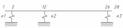
Fig. 1 Line rotor-bearing model

The rotor model has a total of 56 degrees of freedom, Table 1.

Table 1

i	l _i,i+i1	R_i	r_i	R_i+1	r_i+1	M_i	J_di
1	45	45.5	40	45.5	40
2	36	46.5	40	46.5	40
3	41	50	40	50	40
4	47	63	45	124	115
5	40					64.5	3.9
6	195	149.5	146	149.5	146	64.5	3.9
7	27					41.5	2.9
8	170	148.5	145	148.5	145	41.5	2.9
9	28					33.5	2.4
10	28	130	118	90	75	33.5	2.4
11	68	76	55	76	55
12	40	76	48	76	48
13	105	60	48	60	48
14	200	60	48	60	48
15	200	60	48	60	48
16	200	60	48	60	48
17	200	60	48	60	48
18	200	64	54	64	54
19	200	64	54	64	54
20	200	64	54	64	54
21	200	64	54	64	54
22	200	64	54	64	54
23	200	64	54	64	54
24	100	64	54	64	54
25	28.5	66	54	74.5	63.3
26	30	74.5	63.3	85	72.3
27	71	85	72.5	148	140
28						147	7.9

The rotor data are presented in table: i - number of section; l - length of station, mm; R - outer radius, mm; r - internal radius, mm; M - concentrated mass (disk) in i-th section, kg; J - transverse moment of inertia in i-th section, kgm. The station with vanish volumes of radius are given as absolutely stiff.

Problem 1. Investigate a method of reanalysis when all bearing stiffness are increased by one order. As basis use a set of mode shapes, obtained with the next bearing stiffness k₁=k₂=k₃=10⁷ N/m.

Such a problem, for example, is connected with large non-linearity of dampers, due to a large amplitude whirl.

The results of eingenvalue problem, obtained by means of reanalysis and transfer matrix method are presented in Table 2.

Table 2

	Natural frequencies, min^-1
	Basis	Rotor model k₁=k₂=k₃=10⁸ N/m.
N	k₁=k₂=k₃=10⁷ N/m.	Modes in basis (problem size)	Direct
		5	10	20	30	solution
1	2156	3696	3682	3680	3680	3681
2	2667	6539	6533	6531	6530	6530
3	3491	9565	9462	9439	9437	9434
4	6989	10860	10680	10620	10620	10620
5	13680	17720	17270	17220	17220	17220
6	26060		27200	27180	27180	27180
7	44950		45260	45230	45230	45230
8	67060		67396	67380	67380	67390
9	88620		89300	89280	89280	89290
10	111700		112167	112130	112130	112100

To estimate errors the mode shapes were normalized such the sum of the absolute values of elements in modes be equal to one

(5)

The percentage errors in the rotor model modes were computed using a standard expression

(6)

Table 3

	Frequency and mode errors, %
N	Problem size
	5	10	20	30
	freq.	mode	freq.	mode	freq.	mode	freq.	mode
1	0.42	2.16	0.04	0.14	0.00	0.02	0.00	0.01
2	0.15	1.02	0.07	0.15	0.03	0.04	0.02	0.03
3	1.39	5.66	0.29	2.93	0.05	0.39	0.03	0.24
4	2.30	12.48	0.69	4.11	0.09	0.50	0.05	0.30
5	2.97	18.36	0.34	1.78	0.04	0.14	0.03	0.1
6			0.09	1.43	0.01	0.11	0.01	0.08
7			0.02	1.02	0.00	0.07	0.00	0.05
8			0.01	1.23	0.00	0.09	0.00	0.06
9			0.01	1.70	0.00	0.13	0.00	0.05
10			0.01	1.78	0.00	0.11	0.00	0.07

Problem 2. Investigate a method of reanalysis when all bearing stiffness are decreased by one order. As basis use a set of mode shapes, obtained with the next bearing stiffness k₁=k₂=k₃=10⁹ N/m.

The results are presented in Tables 4 and 5.

Table 4

	Natural frequencies, min^-1
	Basis	Rotor model k₁=k₂=k₃=10⁸ N/m.
N	k₁=k₂=k₃=10⁹ N/m.	Modes in basis (problem size)	Direct
		5	10	20	30	solution
1	3926	3684	3746	3703	3690	3681
2	9578	7228	6916	6753	6700	6529
3	21080	11400	10250	9837	9688	9434
4	24860	16990	13470	12120	11203	10620
5	26880	22620	20380	18350	17710	17220
6	41530		29180	27710	27400	27180
7	52430		45790	45410	45300	45230
8	69580		67930	67590	67450	67390
9	94260		90200	89600	89390	89290
10	116600		112800	112320	112190	112100

Table 5

	Frequency and mode errors, %
N	Problem size
	5	10	20	30
	freq.	mode	freq.	mode	freq.	mode	freq.	mode
1	4.90	18.70	1.80	5.87	0.61	2.43	0.43	1.46
2	10.70	18.64	5.90	6.09	3.40	3.62	2.60	2.90
3	20.80	114.70	8.60	52.18	4.20	34.70	2.60	17.13
4	60.00	81.74	26.90	68.44	14.10	43.88	5.50	20.09
5	31.40	92.27	18.30	40.34	6.60	15.11	2.90	6.26
6			7.40	22.36	1.90	7.68	0.80	3.36
7			1.20	8.93	0.40	2.88	0.15	0.98
8			0.80	10.12	0.30	3.45	0.10	0.81
9			1.00	13.83	0.36	4.33	0.11	0.91
10			0.50	13.88	0.17	3.67	0.05	0.72

Comparing the results of problems 1 and 2, it should be noted that the basis, obtained with lower bearing stiffness and used in the reanalysis of rotor model appear to be with less errors than the basis, obtained with high stiffness coefficients.

3. Component mode synthesis

Due to the component mode synthesis a large system is partitioned by a truncated set of vibration modes (basis), obtained in any method. The subsystems are coupled through modal connecting elements into a set of complex system equations of reduced order. The main equations of motion of dynamic system are represented in [ 2 ] and [ 3 ]. The modal equations of a dynamic system, consisting of w - subsystems is of the form

+ = ;

Consider a linear element, connecting the s-th degree of freedom in subsystem p and the t-th degree of freedom in subsystem q. The contribution in the modal stiffness and the damping of modal equation are

(8)

where

(9)

The total effect due to several linear linking elements is the sum of all individual contributions.

This method is a powerful tool in determining the dynamic response of large structures. However, certain quantity of errors is always introduced in some modes less the number of degrees of freedom be presented in system. To estimate the accuracy of component mode synthesis with regard to rotor systems consider two problems.

Problem 3 Using a component mode synthesis determine the frequencies and free modes of a rotor, consisting of two coaxially mounted shafts, Fig.2.

Fig. 2 Line rotor system model

Disregarding the intershaft linking elements distinguish two subsystems. Geometrical data are tabulated in Table 6. The stiffness coefficients of intershaft links and supports are k1=k2=k3=0.1x10⁹ N/m.

Table 6

Subsystem 1
i	l_i,i+1,mm	R_i,mm	r_i,mm	R_i+1, mm	r_i+1, mm
1	250	100	0	100	0
2	250	100	0	100	0
3	250	100	0	100	0
4	250	100	0	100	0
Subsystem 2
i	l_i,i+1,mm	R_i,mm	r_i,mm	R_i+1, mm	r_i+1, mm
1	250	100	0	100	0
2	250	100	0	100	0
3	250	100	0	100	0
4	250	100	0	100	0
5	250	100	0	100	0
6	250	100	0	100	0

The eigenvalue problem has been solved for each subsystem using a finite element method. The determined sets of modes were used in the modal synthesis. Direct computing of the whole rotor system was performed by transfer matrix method developed for multi-shaft rotor systems.

The results of both the component mode synthesis and the transfer matrix method are compared in Table 7.

The analysis of computing results shows good accuracy of the method for multi-shaft rotor systems. The percentage error in frequencies is less than 1% according to data in Table 7. Next conclusion - in practice for linear systems the errors depend insignificantly on the number of modes. The modes with the operating speed range are sufficient to obtain good accuracy. The largest error in the modes due to modal truncation is less than 1% even for the problem size of 3+3.

Table 7

	Frequencies, min^-1
			Rotor model
N	Subsystem 1	Subsystem 2		Modal synthesis
			Direct solution	Problem size
				3+3	5+5
1	8858	6981	7726	7725	7724
2	22627	14081	14335	14350	14343
3	67951	36614	14773	14780	14771
4	130797	73206	24101	24136	24108
5	204853	117687	36929	36925	36924

Problem 4. Using a component mode synthesis determine the frequencies and free modes of a single shaft rotor with three supports, Fig 1. The solution must be computed with the basis sets for two subsystems obtained by breaking the rotor in the second support point.

The results are presented in Table 8.

Table 8

	Frequency and mode errors, %
N	Problem size
	20% (5+7)	50% (12+17)	100% (24+34)
	freq.	mode	freq.	mode	freq.	mode
1	0.15	3.51	0.02	0.76	0.00	0.00
2	2.78	9.26	0.57	1.95	0.00	0.00
3	0.07	2.14	0.00	0.36	0.00	0.00
4	4.09	11.97	1.02	2.75	0.00	0.00
5	11.60	22.51	2.51	5.35	0.00	0.00
6	0.81	8.85	0.26	2.60	0.00	0.00
7	6.59	44.87	2,17	8.04	0.00	0.00
8	7.93	95.95	0.69	26.48	0.00	0.00
9	0.90	19.21	0.33	6.22	0.00	0.00
10	22.35	139.06	0.03	13.93	0.00	0.00

It should be noted that the errors depend essentially on the number of truncated modes. An acceptable result for the first four modes of examined rotor system is observed for a problem size of 12+17 (50% of modes). In this case the percentage frequency errors are less than 1% and the mode errors are less than 3%.

4. The dynamic transformation method in modal methods

The accuracy of modal methods can be reached by increasing the number of modes in the basis. However, in this case the dynamic analysis will require a solution of large order sets of modal equations of motion and may be time consuming. Therefore it’s necessary to use methods, which reduce the truncation errors without increasing the problem size.

One of such methods is a dynamic transformation method. The concept of this method has been developed in [ 4 ]. The dynamic transformation method is set up from the full differential equations of motion and takes into account the influence of higher modes which are not in the basis.

For undamped system of several degrees of freedom, the equation of motion in modal form becomes as

(10)

Partitioned the coordinates in two parts: retained modes in basis and truncated modes . The truncated modes are higher modes, extracted from equations of motion. As a result of this action there is a sum of errors.

For both types of modal coordinates an equation of motion is

(11)

Vector can be written as

(12)

where

(13)

Designate a dynamic transformation matrix by [T]. Then from equation

(14)

obtain a dependence between [R] and [T]

(15)

Hence we can write a dynamic equation of motion in terms of and [T].

(16)

When in equation =0, this method is reformed to the static transformation method of Guyan [ 5 ]. The dynamic transformation method can easily be implemented in any modal method.

Since the formation of matrix [ T ] is not consuming process, in most cases of a dynamic transformation method we can take into account all truncated coordinates.

Consider the implementation of a dynamic transformation method in the modal reanalysis of locally modified structures and in the component mode synthesis.

Problem 5 Using a method of modal analysis of locally modified structures and a dynamic transformation method determine natural frequencies and modes for a rotor model with bearing stiffness coefficients k₁=k₂=k₃=10⁹ N/m, Fig 1. As a basis use the set of mode shapes, obtained with bearing stiffness k₁=k₂=k₃=10⁷ N/m. Determine the errors of natural frequencies and modes.

For computations 20% of mode shapes were used in the basis (problem size of 11). A dynamic transformation method use 20%, 50% and 100% of truncated modes in succession.

The result of this investigation is shown in Table 9.

Table 9

	Frequency error, %	Mode error, %
N	DT problem size	DT problem size
	0 %	20 %	50 %	100 %	0 %	20 %	50 %	100 %
1	0.06	0	0	0	0.25	0.20	0.22	0.23
2	0.14	0.03	0	0	0.61	0.55	0.55	0.56
3	0.51	0.20	0.01	0	3.70	1.72	1.92	1.97
4	6.17	0.67	0.13	0.05	15.04	12.32	12.77	12.83
5	0.66	0.36	0.02	0	12.90	2.15	1.390	1.35
6	1,20	0.18	0.04	0.02	9.50	5.57	6.03	6,11
7	5.70	0.63	0.19	0.13	18.24	15.80	15.71	15.71
8	1.47	0.15	0.07	0.06	18.00	11.31	11.03	11.00
9	1.20	0.23	0.15	0.14	16.68	13.91	13.82	13.81
10	1.40	0.40	0.33	0.31	24.01	20.42	20.20	20.17

It should be noted that the application of a dynamic transformation method reduces the errors of natural frequencies; however the errors of mode shapes are practically without changes.

Problem 6. Using a component mode synthesis and a dynamic transformation method determine natural frequencies and modes for a single rotor with three supports, Fig 1. The solution must be computed with the basis sets for two subsystems obtained by breaking the rotor in the second support point.

20% mode shapes were included in the basis of each subsystem. The results obtained both for dynamic transformation method and without it are presented in Table 10.

Table 10

	Frequency error, %	Mode error, %
N	DT problem size	DT problem size
	0 %	20 %	50 %	100 %	0 %	20 %	50 %	100 %
1	0.15	0.04	0.01	0	3.51	1.08	0.43	0.13
2	2.78	0.81	0.31	0	9.26	2.82	1.23	0.62
3	0.07	0.01	0.05	0	2.14	0.56	0.25	0.15
4	4.09	1.38	0.55	0	11.94	4.04	2.01	2.13
5	11.60	3.45	1.36	0.20	22.51	7.82	3.90	2.53
6	0.81	0.34	0.15	0	8.85	3.20	1.45	1.13
7	6.59	3.04	1.30	0.10	44.87	13.49	7.49	5.92
8	7.03	1.14	0.37	0.03	95.95	39.44	16.78	6.26
9	0.90	0.46	0.26	0.08	19.21	7.74	6.30	7.14
10	22.35	7.02	3.66	1.77	139.06	127.66	124.60	122.99

As a result of this investigation we conclude that a dynamic transformation method reduces the errors of natural frequencies but the errors of mode shapes were remained large again.

5. The inertial loading method

Here we suggest a new method allowing to considerably increase the accuracy both when computing the frequencies and in forming the modes practically without increasing the machine computing time. This is an inertial loading method.

The concept of this method is in introduction into the basis set of frequencies and mode shapes of such modes and by those degrees of freedom where changes are taking place.

In using the modal method for locally modified structures we introduce additional inertial loading of a dynamic system by degrees of freedom where local changes of the elastic or inertial parameter are taking place. In using the modal synthesis we load the boundaries of subsystems in places of their connections.

Then we calculate the basis set frequencies and mode shapes. The included load is then excluded from a dynamic system at a final stage of calculations by means a locally modified structure method.

Study the result of inertial loading method in the early considered problems 5 and 6.

Problem 7. Using a method of modal analysis of locally modified structures and an inertial loading method determine natural frequencies and modes for the rotor model with bearing stiffness coefficients k₁=k₂=k₃=10⁹ N/m, Fig 1. As a basis use the set of mode shapes, obtained with bearing stiffness k₁=k₂=k₃=10⁷ N/m. Determine the errors of natural frequencies and modes.

In places of location of all three supports when calculating the initial set of mode shapes we added an inertial element of 10² kg mass. When passing over to a new set with a support stiffness 10⁹ N/m, this load was removed. Table 11 illustrates the results of calculations.

One can observe a considerable increase of accuracy in our calculations both in natural frequency and modes. So, already at 20% the first nine modes result a very high accuracy. Any specification of higher mode shapes requires widening of the basis.

Table 11

	Frequency error, %	Mode error, %
N	Problem size	Problem size
	10 %	20 %	10%	20 %
1	0.03	0.00	1.40	0.09
2	0.04	0.00	0.40	0.03
3	0.15	0.00	0.16	0.00
4	0.60	0.03	2.57	0.05
5	0.76	0.03	3.42	0.14
6	5.60	0.05	36.90	0.41
7		0.18		1.07
8		0.03		1.35
9		0.11		2.56
10		0.21		32.90

Problem 8. In solving the problem of synthesis the compatible boundaries of subsystems were loaded by an inertia moment J_d , equaling 10 kgm² and at a final stage of computations this load was removed. Decomposition was carried out by 20% of modes from each subsystem. The results, given in Table 14, show considerable increase of accuracy, especially by the mode shapes.

Table 13

	Frequency error, %	Mode error, %
N	without loading	with loading	without loading	with loading
1	0.15	0.00	3.51	0.07
2	2,78	0.01	9.26	0.11
3	0.07	0.01	2.14	0.12
4	4.09	0.07	11.97	0.54
5	11.60	0.23	22.51	1.41
6	0.81	0.01	8.85	2.95
7	6.59	0.20	44.87	2.42
8	7.93	0.45	95.95	4.01
9	0.90	10.40	19.21	45.50
10	22.35	82.50	139.06	105.00

A large error by the last modes is connected with insufficient amount of modes in the basis.

6. CONCLUSIONS

The results of studies on the accuracy of modal methods give us a possibility tj make the following main conclusions.

1. A method of reanalysis of locally modified structures allows to reduce a time of computation as compared to direct methods.

2. It is preferable to use in the method of reanalysis of locally modified structures a basis obtained for minimum possible stiffness values of the rotor supports within the range of their possible change.

3. In using of modal reanalysis method to obtain satisfactory results we may recommend to set up a basis by the number of modes from the range not less than 2, 3 times exceeding the frequency range in which a solution is sought for.

4. A modal synthesis, used for solving the problems of second type (Fig 2), may give somewhat worse results as against the problem of the first type (Fig 1) and hence in every particular case a preliminary estimate of the accuracy is required for the results being obtained in order to define the boundaries of the basis set.

5. Methods of dynamic transformation and inertial loading considerably reduce the errors of modal methods, connected with a truncation of higher mode shapes.

6. High accuracy of the results and simplicity make the inertial loading method more preferable as compared with a dynamic transformation method.

LITERATURE

1. M.K. Leontiev. Modal analysis in research of dynamic behavior of complicated elastoinertial aircraft GTE systems. In System analysis of machines dynamics and durability. Irkutsk polytechnic institute.Irkutsk,1988

2. M.K. Leontiev. Modal analysis in research of dynamic behavior of complicated aircraft GTE systems. Aviation technics, Moscow, N1,1988

3. Li, D.F., Gunter, E.J. Component mode Synthesis of Large Rotor Systems, Trans. ASME, Vol. 104, July 1982, pp 552-560.

4. E.J.Kuhar, C.V.Sthale. Dynamic Transformation Method For Modal Synthesis, AIAA Journal, vol. 12, №5. 1974. pp 672-676.

5. R.J. Guyan Reduction of Stiffness and Mass Matrices, AIAA Journal, vol. 3, №2, 1965, pp. 380-386.

ROTOR DYNAMICS OF TURBOMACHINERY

Engineering & Consulting Centre for Dynamic Problems in Rotating Machinery